Simulating Models with Infobiotics Workbench

In this section we will show, step-by-step, how to perform stochastic simulations of models and analyse the results of these simulations.

Simulating simple gene regulation

We will start by using the model of simple gene regulation implemented before in CellDesigner. For this model, we will show how to calculate the response time of this gene regulatory network. To simulate the model, we will use the Infobiotics Workbench (IBW). We now take a look at some screenshots of IBW.

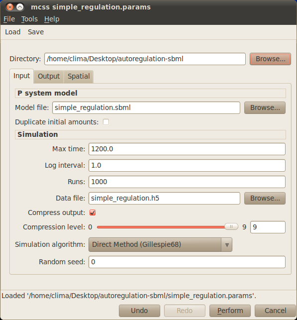
The simulation control window of IBW where the parameters for the simulation are entered:

The simulation results tab, which opens automatically once the simulation has finished:

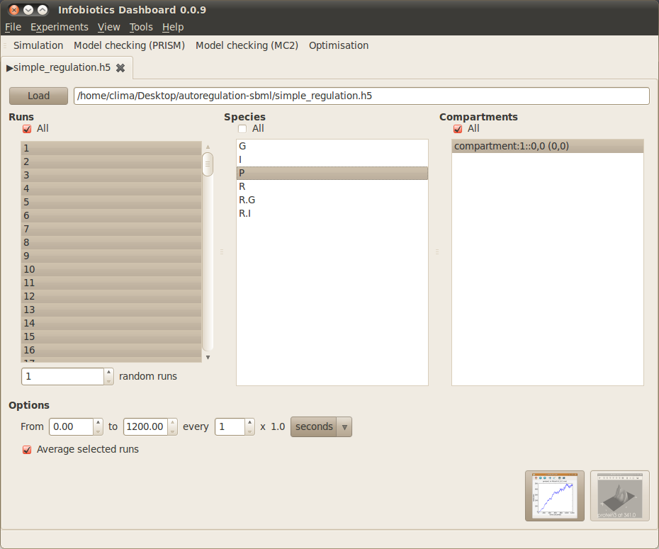
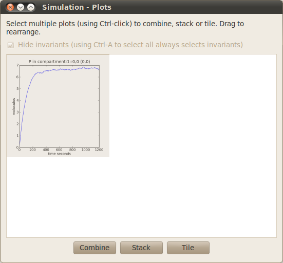
The simulation results tab is used to select the runs, species and compartments which you want to plot graphs of. Once these have been selected, a graph overview window will open, which will show and allow further manipulation of these graphs:

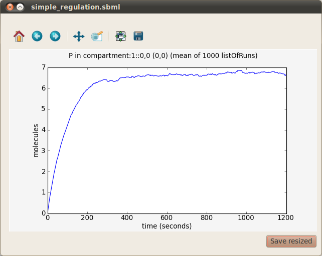
The final graph you should obtain from which you will be able to calculate the response time is:

Follow the steps below and you should end up with something very similar:

1. Open the simulation window by clicking on Simulation.
2. Set the name of the model file in the Model file text box in the simulation control window. Since we are simulating the simple gene regulation model implemented before, you should enter simple_regulation.sbml for the name of model file.
3. Set the time in seconds you want to simulate the model for. We will be simulating each simulation run for 20 minutes i.e. 1200 seconds, so enter 1200 in the Max time text box. Set also the Log interval to 1.
4. Set the number of simulation runs of the model you want to perform. With stochastic simulation, due to the random fluctuations inherent in this modelling approach, it is common to perform a number of simulation runs and average the number of molecules of each species over these runs to gain an insight into the average behaviour of the model. We will do this for the simple regulation model and average the species levels over 1,000 runs, so enter 1000 in the Runs text box.
5. Set the name of the data file you want to save the simulation results in. Simulation results are stored in HDF5 format (a scientific data storage standard), whose files usually use the ‘.h5’ extension. Since we are simulating the simple gene regulation model, in the Data file text box enter simple_regulation.h5 for the data file filename.
6. Leave the rest of the parameters with their default values.
7. Simulate the model by clicking on the Perform button. A progress bar should appear showing the progress of the simulation. Once all the simulation runs have finished (this may take around a minute) the simulation results tab should appear.
8. Select the runs you want to use when plotting graphs. In the simulation results window there are three panes, the left hand one of which (titled Runs) lists the runs performed during the simulation. We want to use all these runs to calculate the average levels of species in the simulation. so check the All box at the top of this pane. All the runs in the list should now be highlighted.
9. Select the species you want to plot graphs for. In the middle pane (titled Species) of the simulation results window you’ll see a list of species in the simple gene regulation model. We are interested in the levels of the protein P which is produced by the gene, so highlight P in the list of species by left clicking it once.
10. Select the compartments you want to plot graphs for. In the right hand pane (titled Compartments) you’ll see a list of compartments. Since there is only one compartment in the simple gene regulation model there will only be one entry (called compartment:1::0,0) in this list. Highlight this entry in the list of compartments by left clicking it once.
11. Click on the first button located at the bottom right corner of the simulation tab. The graph overview window should now appear.
12. Open the plot of protein P vs. time in a separate window by pointing to this graph in the graph overview window and left clicking it once to highlight it. Now click on the Tile button. A new window containing this graph should open. You can resize this window, zoom in and out, use the cursor to determine the location of points of the graph, and save the resulting graph.
13. Determine the response time of the simple gene regulation model. Remember, the response time is defined as the time taken to reach half the steady-state level. So, first determine the steady-state level by examining the graph of protein P vs. time. Now examine the graph to find the time at which the level of protein P reaches half this steady-state level.

Congratulations - you have now performed a stochastic simulation of a simple gene regulation network and calculated its response time!

Simulating negative and positive autoregulation

Simulate and determine the response times of the other two models of gene regulation (negative autoregulation and positive autoregulation).

You now should be able to answer the following questions:

1. Which of the three motifs (simple regulation, negative autoregulation, and positive autoregulation) gives the fastest response time and which one the slowest?
2. Can you explain why this is the case? (looking at the levels of the other species).
3. What other differences do you notice in the production of protein P between the three models?