Quick Start
In this quick start we will walk through an example based on gene negative autoregulation (NAR) to explain the basics of getting started with the Infobiotics Workbench. Alternatively you can follow our video tutorial.
- First you need to download and install Infobiotics Workbench from this link.
- Download this example containing the NAR model and unzip it to your favourite location.
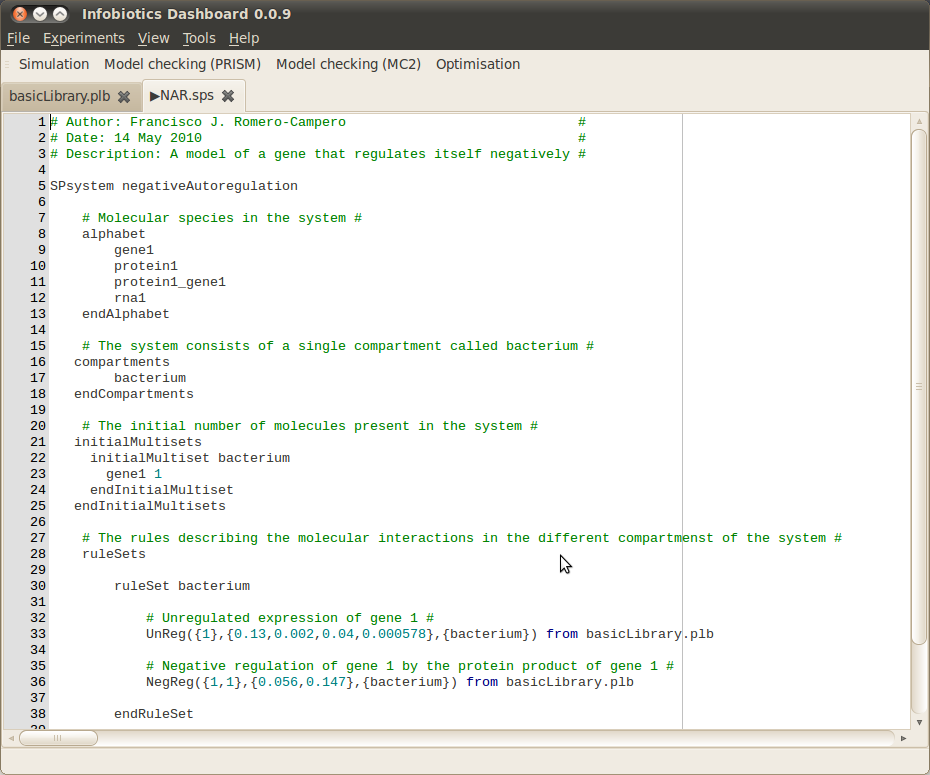
- Open the Infobiotics Workbench by double clicking on the corresponding icon located on your desktop (Windows) or by choosing it from your Applications menu (Mac/Linux). The following window will appear showing the different components: simulation, model checking (PRISM and MC2) and optimisation - without the open model files shown.
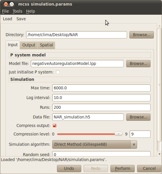
- Click on the Simulation button on the toolbar to open up the dialog window below allowing you to specify your simulation parameters.
- Load the simulation parameter file simulation.params by selecting Load from the dialog toolbar and navigating to the location of the NAR model.
- Run your simulations by clicking on the Perfom button at the bottom of the simulation dialog window.
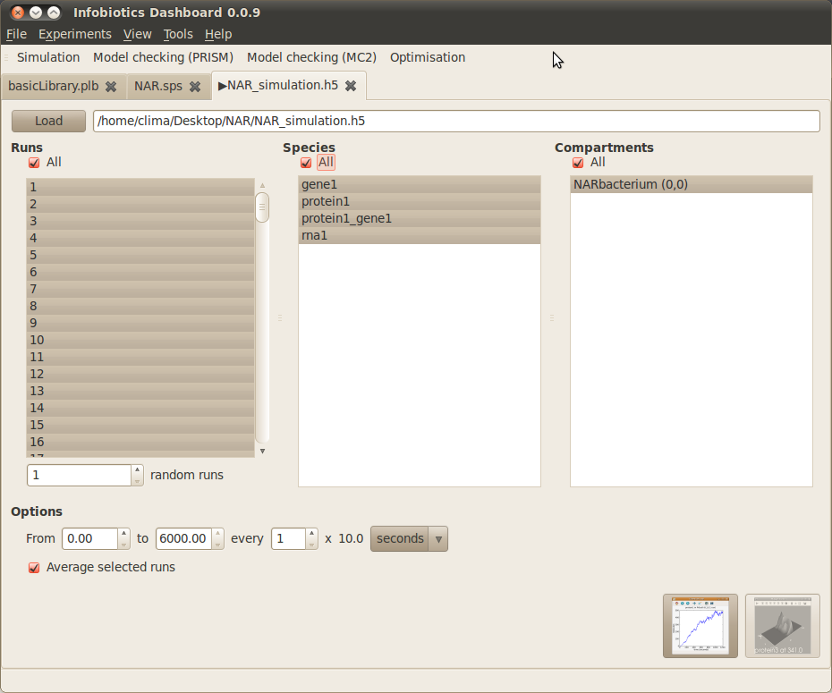
- Once your simulations have finished the following tab will appear to allow you to plot the results.
- Plot the average number of molecules over time for all species in all compartments by checking All under Runs, Species and Compartments, then clicking on the first button (‘timeseries’) in the bottom right corner.
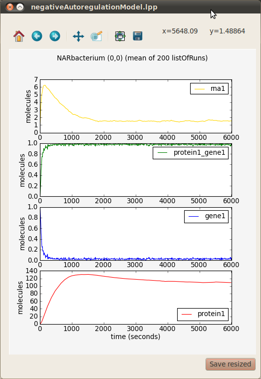
- A preview window will appear that allows you to combine the various timeseries in different ways. Select all the graphs (Ctrl-A) and click the Stack button to view each timeseries with the same time axis but individual molecules axes.
The Infobiotics Workbench is not limited to performing simulations, you can apply other techniques to analyse and manipulate your models. Visit the links below if you are interested in the different components of our workbench.
For more details on how to use the Infobiotics Workbench you can read our tutorials.


