Model Formal Analysis using Model Checking
The Infobiotics Workbench allows you to analyse probabilistic spatio-temporal properties of your models using two model checkers PRISM and MC2. In this tutorial we will use our running example based on autoregulation to illustrate this feature. Alternatively, you can see our video tutorial.
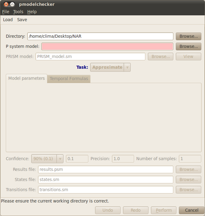
Click on the Model checking (PRISM) tab located on the upper menu bar of the infobiotics dashboard to start up the dialog window below that will allow you to specify your model properties and the necessary parameters.
First of all, you need to specify your working directory. Click on the first Browse button at the top right corner of the dialog window and navigate to the folder where the files comprising the autoregulation model are located. Next you need to introduce the name of the file containing your P system model (lpp file). In our running example we will analyse the behaviour of single cells carrying three different gene regulatory mechanisms, gene unregulated expression, positive autoregulation and negative autoregulation. This model is specified in the file individualCells.lpp, please click on the corresponding Browse button and select this file.
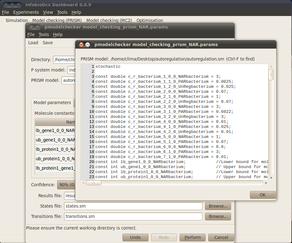
Infobiotics workbench allows you to perform different Tasks in order to analyse properties of your model. The first task you must perform is to Translate your model into the specific language used by the model checker PRISM. In order to do this you need to provide a name for the PRISM model. Please type autoregulation.sm in the corresponding box. This model will be created after you click on the Perform button located at the bottom of the model checking dialog window. The PRISM model can be inspected by clicking on the View button next to the PRISM model box. You should see the following windows:
Typically, a PRISM model has a set of parameters representing the upper and lower bounds for the number of the different molecular species in the system. The stochastic constants associated with rules can also be model parameters. The values for these parameters must be specified using the Model parameters tab in the model checking dialog window and the box enumerating the Model constants. Notice that a brief description of each parameter is provided to assist you in choosing appropriate values for them. For our case study, please click on the Value box to set all the lower bounds for the different number of molecules to 0, the upper bounds for gene1 and protein1_gene1 to 1 and the rest of upper bounds to 1000.
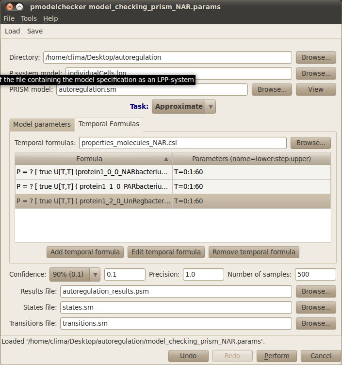
The properties to be analysed can be specified using the Temporal Formulas tab. Click on it and give a name to the file where the properties will be saved, for example type properties.csl. New formulas can be added by clicking on the Add temporal formula button. Existing formulas can be modified by clicking on the Edit temporal formula or deleted by clicking of the Remove temporal formula button.
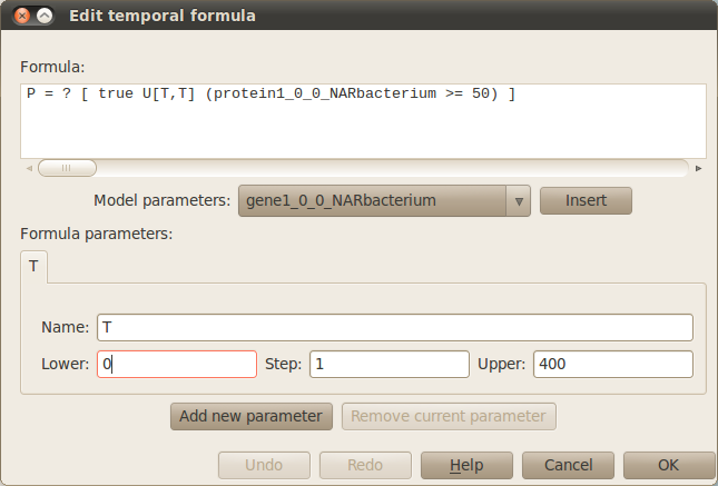
When specifying or editting the formulas that represent your model properties the following window will pop up. This window allows you to specify/edit your formula, add/edit/remove parameters used in your properties and insert model parameters in your formula using the corresponding drop down list and Insert button. In our example, we analyse the response time (time needed to reach half the maximal expression of gene) of the different regulatory mechanisms represented in the autoregulation case study. The temporal formulas associated with the response time computes the probability of the number of protein1 molecules at positions (0,0), (1,0) and (2,0) in the comparments NARbacterium, PARbacterium and UnRegbacterium to exceed 50 molecules at time T where this parameter varies from 0 to 400 with a step of 1 as the following figure shows:
For more details on how to specify your model properties using temporal formulas you can visit the PRISM web site.
In our case study we will approximate the probabilities associated with the above temporal formulas. For this, please choose Approximate from the drop down list specifying the different Tasks that can be performed. Note that Verify is also available to analyse properties, nevertheless this task is computationally very expensive and is only feasible for very small systems. You also need to specify the Number of samples or simulation runs of your model that will be used in the approximation of the propabilities associated with your model properties. Please type 1000 runs for our example.
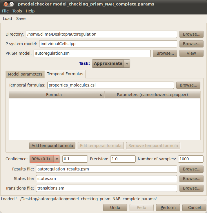
Finally, the Results file containing the output of the model checking analysis must be provided, autoregulation_results.sm for our example. Your model checking dialog window should look similar to the figure below:
Other parameters such as the states/transitions files and precision/confidence of the approximation can be specified. Although they are not relevant in our running example they can be of interest for your analysis, see our documentation for more details.
You can save your model checking parameters by clicking on the Save button located on the upper menu bar of the model checking dialog window. These can be loaded in order to reproduce your model checking settings by clicking on the Load button and choosing the file containing your parameters.
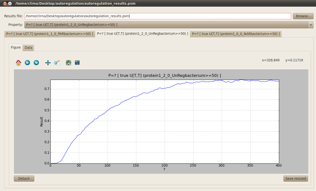
In order to run the analysis of your model properties according to the parameters you have introduced click on the Perform button located at the bottom right corner. Once the model checking finishes the following tab appears on the main window to allow you to see the results for your different model properties.
A graph is generated for each temporal formula representing your model properties. These graphs can be detached so you can see the results from the different properties one next to the other by clicking on the Detach button at the bottom right corner.
The Infobiotics Workbench also allows you to analyse properties of your models using MC2. In this case you are able to reuse previous simulations performed for your model. Please click in the link below for a short tutorial on how to use the model checker MC2 integrated in Infobiotics Workbench.
